Image Processing and Neural Networks Intuition: Part 3

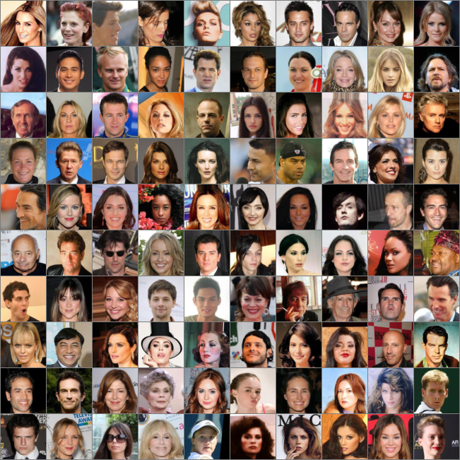
In the last article, we saw how to implement logistic regression as a neural network with single neuron. In this article, we will explore how we can use Multi layered Neural Networks(multiple layers of neurons) for classifying images. We will continue exploring the same problem from last article i.e predicting the gender of the celebrity from the images.

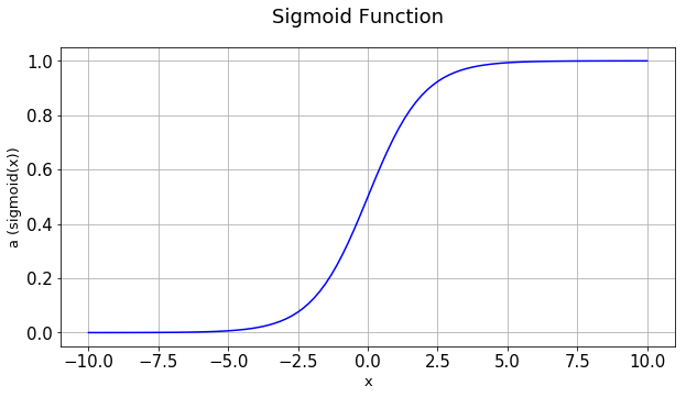
Let’s quickly recap the structure of one neuron neural network. It has mainly two components, Z and A. Z is the linear combination of inputs and A is a non-linear transformation on Z. We used sigmoid function as the non-linear transformation.

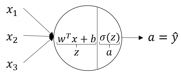
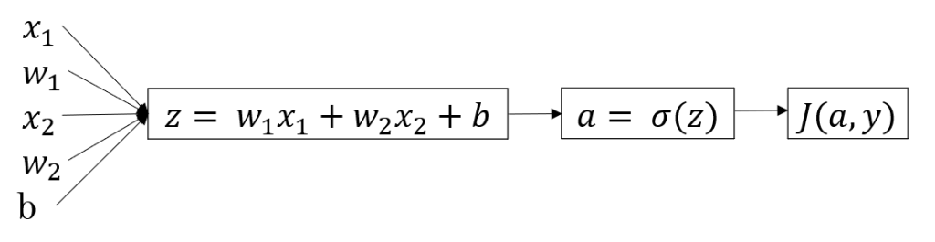
The above image shows the layout of a single neuron. x1,x2,x3 are the inputs, z is the linear function of inputs with weights W(a vector) and a is the sigmoid function of z.

Training of single neuron neural network using gradient descent involves the following steps:

1) Initialize parameters i.e W and b

2) Forward Propagation: Calculate Z and A using the initialized parameters

3) Compute cost

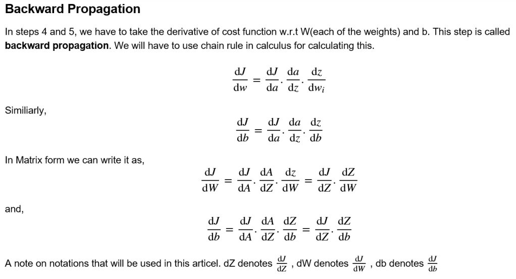
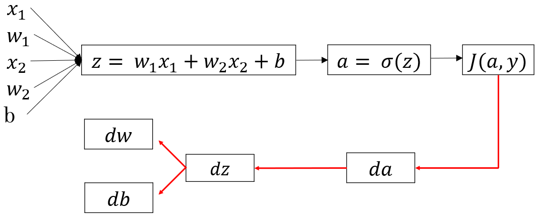
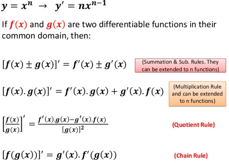
4) Backward propagation: Take gradient(derivative) of cost function with respect to W and b

5) Use the gradients to update the values of W and b

6) Repeat steps 2 to 5 for a fixed number of times

Cost is given as :

Derivatives used in backward propagation:
dA =  = 

dZ =  == A-Y

dW =  = 

db =  = 

where  is the transpose of X and the function to calculate a is sigmoid.

Activation Functions

Important point to remeber is that during forward propagation, we need to calculate z and a. Till now we have only used sigmoid as the function to calculate a. But we can also use other functions for a. These functions for a is called activation functions. Activation functions take z as the input and apply some form of non-linear function. Other commonly used activation functions are hyperbolic tangent, relu and leaky relu.

Tanh(hyperbolic tangent) = 

Relu(Rectified Linear Units) = 

Leaky relu = 

Cost will remain the same for any activation function. But in back propagation, dZ will vary for different activation functions. Rest of the derivatives will be the same. The reason for change is  will vary depending on the activation function.

For sigmoid,  = 

For tanh,  = 1-

For relu,  = (0, if z < 0; 1, if z >= 0)

For leaky relu,  = (0.01, if z < 0; 1, if z >= 0)

From the above equations , now you can see for sigmoid function how  = dZ, became A-Y.

Multi Layered Neural Networks

Architecture of Multi Layered neural networks will look something like this.

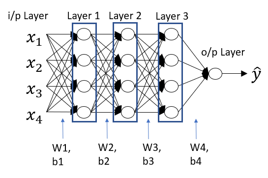
The inputs can be considered as input layers or layer 0. The last layer is the output layer. All the middle layers are called hidden layers i.e layer1,2 and 3. It’s called hidden because not much is known about what is happening inside these layers. Many people call neural networks as black box algorithm for the same reason. Understanding the working of neurons in the hidden layers is still a research area.

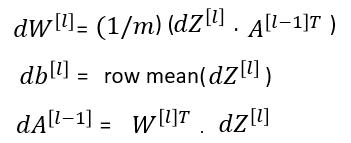
The calculations used for a single neuron can be expanded and generalized for multiple layers containing multiple neurons. Following figure shows the generalized calculations for each layer. It includes calculations for forward propagation and backward propagation.

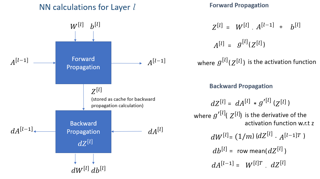
The above quations, summarize the calculations for each layer in neural networks. The superscript [] denotes the layer L. For every layer, after back propagation, weights and bias are updated as follows:

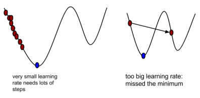
where  is the learning rate.

The number of layers and number of neurons in each layer is a hyperparameter to tune. Generally, more number of layers you have, you will need less number of neurons in each layer. However, more number of layers will slow down the computations as well.

Gender Prediction from Celebrity images

Now let’s implement multi layered neural nets to solve our problem of predicting the gender of the celebrity from the image. We will use leaky relu activation for the hidden layers, three of them, and sigmoid activation for the output layer. We will continue from where we stopped in the last article.

First let’s define our activation functions, sigmoid and relu, which will take Z as the input. Sigmoid function = 
and leaky relu function = 
where 

In [77]:

def sigmoid(Z):
    """
    Implements the sigmoid activation in numpy
    
    Arguments:
    Z -- numpy array of any shape
    
    Returns:
    A -- output of sigmoid(z), same shape as Z
    cache -- returns Z as well, useful during backpropagation
    """
    
    A = 1/(1+np.exp(-Z))
    cache = Z
    
    return A, cache

def relu(Z):
    """
    Implement the RELU function.

    Arguments:
    Z -- Output of the linear layer, of any shape

    Returns:
    A -- Post-activation parameter, of the same shape as Z
    cache -- a python dictionary containing "A" ; stored for computing the backward pass efficiently
    """
    
    A = np.maximum(0.01*Z,Z)
    
    assert(A.shape == Z.shape)
    
    cache = Z 
    return A, cache

Now let’s define functions for backpropagation of activation function. i.e  for sigmoid and relu function.

For sigmoid,  = 

For leaky relu,  = (0, if z < 0; 1, if z >= 0)

We will pass dA and Z(stored as cache) as inputs to the function.

In [43]:

def relu_backward(dA, cache):
    """
    Implement the backward propagation for a single RELU unit.

    Arguments:
    dA -- post-activation gradient, of any shape
    cache -- 'Z' where we store for computing backward propagation efficiently

    Returns:
    dZ -- Gradient of the cost with respect to Z
    """
    
    Z = cache
    dZ = np.array(dA, copy=True) # just converting dz to a correct object.
    
    # When z <= 0, you should set dz to 0 as well. 
    dZ[Z < 0] = dZ[Z < 0]*0.01
    
    assert (dZ.shape == Z.shape)
    
    return dZ

def sigmoid_backward(dA, cache):
    """
    Implement the backward propagation for a single SIGMOID unit.

    Arguments:
    dA -- post-activation gradient, of any shape
    cache -- 'Z' where we store for computing backward propagation efficiently

    Returns:
    dZ -- Gradient of the cost with respect to Z
    """
    
    Z = cache
    
    s = 1/(1+np.exp(-Z))
    dZ = dA * s * (1-s)
    
    assert (dZ.shape == Z.shape)
    
    return dZ

Now let us write a function to intialize the parameters, weights and bias for every layer. Unlike the single neuron case, we have to intialize weights for each layers separately. Weights for every layer will have the shape[no. of neurons in that layer, no. of neurons in the previous layer]. Bias for each layer will have the shape [no. of neurons in that layer,1].

Also, we will initialize weights from a standard normal distribution and multiply by . This is called he intialization. Generally this intialization works well. Biases can be intialized as zeros.

Random intialization of weights are better since it will allow different neurons to learn different aspects of the image. Also, the reason for drawing random numbers from a standard normal distribution(mean=0,std.dev=1) is that this will help in avoiding a problem called exploding or vanishing gradients. I am not going into the details but vanishing gradient in a nutshell means, during backpropagation of a deep neural network, the gradients of the intial layers become so small that they practically cease to update, SImiliarly, Exploding gradients means gradients of intial layers quickly reach a higher number or infinity stopping further learning. Vanishing gradients were one of the reasons why deep learning didn’t become popular until 2006. I didn’t mention earlier why we are using leaky relu activation function for the hidden layers. Leaky relus are better in handling vanishing or exploding gradients.

In [28]:

def initialize_parameters_deep(layer_dims):
    """
    Arguments:
    layer_dims -- python array (list) containing the dimensions of each layer in our network
    
    Returns:
    parameters -- python dictionary containing your parameters "W1", "b1", ..., "WL", "bL":
                    Wl -- weight matrix of shape (layer_dims[l], layer_dims[l-1])
                    bl -- bias vector of shape (layer_dims[l], 1)
    """
    
    np.random.seed(1)
    parameters = {}
    L = len(layer_dims)            # number of layers in the network

    for l in range(1, L):
        parameters['W' + str(l)] = np.random.randn(layer_dims[l], layer_dims[l-1]) * np.sqrt(2/layer_dims[l-1]) #*0.01
        parameters['b' + str(l)] = np.zeros((layer_dims[l], 1))
        
        assert(parameters['W' + str(l)].shape == (layer_dims[l], layer_dims[l-1]))
        assert(parameters['b' + str(l)].shape == (layer_dims[l], 1))

        
    return parameters

Let’s get to the linear forward function. This function will calculate the linear function  , for one layer (for all neurons in the layer) at a time. It will take A from previous layer and W(weight) and b(bias) of current layer as input.

In [79]:

def linear_forward(A, W, b):
    """
    Implement the linear part of a layer's forward propagation.

    Arguments:
    A -- activations from previous layer (or input data): (size of previous layer, number of examples)
    W -- weights matrix: numpy array of shape (size of current layer, size of previous layer)
    b -- bias vector, numpy array of shape (size of the current layer, 1)

    Returns:
    Z -- the input of the activation function, also called pre-activation parameter 
    cache -- a python dictionary containing "A", "W" and "b" ; stored for computing the backward pass efficiently
    """
    
    Z = W.dot(A) + b
    
    assert(Z.shape == (W.shape[0], A.shape[1]))
    cache = (A, W, b)
    
    return Z, cache

Let’s write a function to calculate the derivative values we need in each layer. We already wrote function to calculated Z. In this function we will calculate dW, dB and dA_prev for one layer at a time.

def linear_backward(dZ, cache):
    """
    Implement the linear portion of backward propagation for a single layer (layer l)

    Arguments:
    dZ -- Gradient of the cost with respect to the linear output (of current layer l)
    cache -- tuple of values (A_prev, W, b) coming from the forward propagation in the current layer

    Returns:
    dA_prev -- Gradient of the cost with respect to the activation (of the previous layer l-1), same shape as A_prev
    dW -- Gradient of the cost with respect to W (current layer l), same shape as W
    db -- Gradient of the cost with respect to b (current layer l), same shape as b
    """
    A_prev, W, b = cache
    m = A_prev.shape[1]

    dW = 1./m * np.dot(dZ,A_prev.T)
    db = 1./m * np.sum(dZ, axis = 1, keepdims = True)
    dA_prev = np.dot(W.T,dZ)
    
    assert (dA_prev.shape == A_prev.shape)
    assert (dW.shape == W.shape)
    assert (db.shape == b.shape)
    
    return dA_prev, dW, db

Let’s define a common activation function for forward propagation and backward propagation, which will take activation as one of the input. Depending on the kind of value is passed for activation, the function will do the calculations for sigmoid or leaky relu.

In [19]:

def linear_activation_forward(A_prev, W, b, activation):
    """
    Implement the forward propagation for the LINEAR->ACTIVATION layer

    Arguments:
    A_prev -- activations from previous layer (or input data): (size of previous layer, number of examples)
    W -- weights matrix: numpy array of shape (size of current layer, size of previous layer)
    b -- bias vector, numpy array of shape (size of the current layer, 1)
    activation -- the activation to be used in this layer, stored as a text string: "sigmoid" or "relu"

    Returns:
    A -- the output of the activation function, also called the post-activation value 
    cache -- a python dictionary containing "linear_cache" and "activation_cache";
             stored for computing the backward pass efficiently
    """
    
    if activation == "sigmoid":
        # Inputs: "A_prev, W, b". Outputs: "A, activation_cache".
        Z, linear_cache = linear_forward(A_prev, W, b)
        A, activation_cache = sigmoid(Z)
    
    elif activation == "relu":
        # Inputs: "A_prev, W, b". Outputs: "A, activation_cache".
        Z, linear_cache = linear_forward(A_prev, W, b)
        A, activation_cache = relu(Z)
    
    assert (A.shape == (W.shape[0], A_prev.shape[1]))
    cache = (linear_cache, activation_cache)

    return A, cache

In [20]:

def linear_activation_backward(dA, cache, activation):
    """
    Implement the backward propagation for the LINEAR->ACTIVATION layer.
    
    Arguments:
    dA -- post-activation gradient for current layer l 
    cache -- tuple of values (linear_cache, activation_cache) we store for computing backward propagation efficiently
    activation -- the activation to be used in this layer, stored as a text string: "sigmoid" or "relu"
    
    Returns:
    dA_prev -- Gradient of the cost with respect to the activation (of the previous layer l-1), same shape as A_prev
    dW -- Gradient of the cost with respect to W (current layer l), same shape as W
    db -- Gradient of the cost with respect to b (current layer l), same shape as b
    """
    linear_cache, activation_cache = cache
    
    if activation == "relu":
        dZ = relu_backward(dA, activation_cache)
        dA_prev, dW, db = linear_backward(dZ, linear_cache)
        
    elif activation == "sigmoid":
        dZ = sigmoid_backward(dA, activation_cache)
        dA_prev, dW, db = linear_backward(dZ, linear_cache)
    
    return dA_prev, dW, db

Now let’s define a function to create any number of layers of neurons from the functions we created. Since we have generalized calculations for each layer, we can add any number of layers. This function will do the forward propagation calcuations iteratively for each layer, starting from the input layer and ending with the output layer.

In [21]:

def L_model_forward(X, parameters):
    """
    Implement forward propagation for the [LINEAR->RELU]*(L-1)->LINEAR->SIGMOID computation
    
    Arguments:
    X -- data, numpy array of shape (input size, number of examples)
    parameters -- output of initialize_parameters_deep()
    
    Returns:
    AL -- last post-activation value
    caches -- list of caches containing:
                every cache of linear_relu_forward() (there are L-1 of them, indexed from 0 to L-2)
                the cache of linear_sigmoid_forward() (there is one, indexed L-1)
    """

    caches = []
    A = X
    L = len(parameters) // 2    # number of layers in the neural network. Every layer has a weight and bias, hence the length of the parameter will be double the layers.
    
    # Implement [LINEAR -> RELU]*(L-1). Add "cache" to the "caches" list.
    for l in range(1, L):
        A_prev = A 
        A, cache = linear_activation_forward(A_prev, parameters['W' + str(l)], parameters['b' + str(l)], activation = "relu")
        caches.append(cache)
    
    # Implement LINEAR -> SIGMOID. Add "cache" to the "caches" list.
    AL, cache = linear_activation_forward(A, parameters['W' + str(L)], parameters['b' + str(L)], activation = "sigmoid")
    caches.append(cache)
    
    assert(AL.shape == (1,X.shape[1]))
            
    return AL, caches

Cost is calculated after the prediction from output layer is obtained. The formula for cost is same as in the last article(the same cost works for all binomial classification problems, although it can be generalized to multi-class classification problem).

In [22]:

def compute_cost(AL, Y):
    """
    Implement the cost function defined by equation (7).

    Arguments:
    AL -- probability vector corresponding to your label predictions, shape (1, number of examples)
    Y -- true "label" vector (for example: containing 0 if non-cat, 1 if cat), shape (1, number of examples)

    Returns:
    cost -- cross-entropy cost
    """
    
    m = Y.shape[1]

    # Compute loss from aL and y.
    cost = (1./m) * (-np.dot(Y,np.log(AL).T) - np.dot(1-Y, np.log(1-AL).T))
    
    cost = np.squeeze(cost)      # To make sure your cost's shape is what we expect (e.g. this turns [[17]] into 17).
    assert(cost.shape == ())
    
    return cost

Now let’s define a function to do the backprop calculations for all the layers we created during forward propagation. Each layer calculation is done iteratively, starting from the output layer and ending with the input layer.

In [23]:

def L_model_backward(AL, Y, caches):
    """
    Implement the backward propagation for the [LINEAR->RELU] * (L-1) -> LINEAR -> SIGMOID group
    
    Arguments:
    AL -- probability vector, output of the forward propagation (L_model_forward())
    Y -- true "label" vector (containing 0 if non-cat, 1 if cat)
    caches -- list of caches containing:
                every cache of linear_activation_forward() with "relu" (there are (L-1) or them, indexes from 0 to L-2)
                the cache of linear_activation_forward() with "sigmoid" (there is one, index L-1)
    
    Returns:
    grads -- A dictionary with the gradients
             grads["dA" + str(l)] = ... 
             grads["dW" + str(l)] = ...
             grads["db" + str(l)] = ... 
    """
    grads = {}
    L = len(caches) # the number of layers
    m = AL.shape[1]
    Y = Y.reshape(AL.shape) # after this line, Y is the same shape as AL
    
    # Initializing the backpropagation
    dAL = - (np.divide(Y, AL) - np.divide(1 - Y, 1 - AL))
    
    # Lth layer (SIGMOID -> LINEAR) gradients. Inputs: "AL, Y, caches". Outputs: "grads["dAL"], grads["dWL"], grads["dbL"]
    current_cache = caches[L-1]
    grads["dA" + str(L)], grads["dW" + str(L)], grads["db" + str(L)] = linear_activation_backward(dAL, current_cache, activation = "sigmoid")
    
    for l in reversed(range(L-1)):
        # lth layer: (RELU -> LINEAR) gradients.
        current_cache = caches[l]
        dA_prev_temp, dW_temp, db_temp = linear_activation_backward(grads["dA" + str(l + 2)], current_cache, activation = "relu")
        grads["dA" + str(l + 1)] = dA_prev_temp
        grads["dW" + str(l + 1)] = dW_temp
        grads["db" + str(l + 1)] = db_temp

    return grads

Let’s write a function to update the parameters using the calculated gradients from backprop. This function can actually be combined in the backprop step. However, to enhance understanding let’s write it separately.

In [24]:

def update_parameters(parameters, grads, learning_rate):
    """
    Update parameters using gradient descent
    
    Arguments:
    parameters -- python dictionary containing your parameters 
    grads -- python dictionary containing your gradients, output of L_model_backward
    
    Returns:
    parameters -- python dictionary containing your updated parameters 
                  parameters["W" + str(l)] = ... 
                  parameters["b" + str(l)] = ...
    """
    
    L = len(parameters) // 2 # number of layers in the neural network

    # Update rule for each parameter. Use a for loop.
    for l in range(L):
        parameters["W" + str(l+1)] = parameters["W" + str(l+1)] - learning_rate * grads["dW" + str(l+1)]
        parameters["b" + str(l+1)] = parameters["b" + str(l+1)] - learning_rate * grads["db" + str(l+1)]
        
    return parameters

Time to put everything together and create a single function for Multi layered neural network. Just to remind, the steps involved are:
1) Initialize parameters i.e W and b
2) Forward Propagation: Calculate Z and A using the initialized parameters
3) Compute cost
4) Backward propagation: Take gradient(derivative) of cost function with respect to W and b
5) Use the gradients to update the values of W and b
6) Repeat steps 2 to 5 for a fixed number of times(num_iterations)

In [82]:

def L_layer_model(X, Y, layers_dims, learning_rate = 0.0075, num_iterations = 3000, print_cost=False):
    """
    Implements a L-layer neural network: [LINEAR->RELU]*(L-1)->LINEAR->SIGMOID.
    
    Arguments:
    X -- data, numpy array of shape (number of examples, num_px * num_px * 3)
    Y -- true "label" vector (containing 0 if cat, 1 if non-cat), of shape (1, number of examples)
    layers_dims -- list containing the input size and each layer size, of length (number of layers + 1).
    learning_rate -- learning rate of the gradient descent update rule
    num_iterations -- number of iterations of the optimization loop
    print_cost -- if True, it prints the cost every 100 steps
    
    Returns:
    parameters -- parameters learnt by the model. They can then be used to predict.
    """

    np.random.seed(1)
    costs = []                         # keep track of cost
    
    # Parameters initialization.
    ### START CODE HERE ###
    parameters = initialize_parameters_deep(layers_dims)
    ### END CODE HERE ###
    
    # Loop (gradient descent)
    for i in range(0, num_iterations):

        # Forward propagation: [LINEAR -> RELU]*(L-1) -> LINEAR -> SIGMOID.
        ### START CODE HERE ### (≈ 1 line of code)
        AL, caches = L_model_forward(X, parameters)
        ### END CODE HERE ###
        
        # Compute cost.
        ### START CODE HERE ### (≈ 1 line of code)
        cost = compute_cost(AL, Y)
        ### END CODE HERE ###
    
        # Backward propagation.
        ### START CODE HERE ### (≈ 1 line of code)
        grads = L_model_backward(AL, Y, caches)
        ### END CODE HERE ###
 
        # Update parameters.
        ### START CODE HERE ### (≈ 1 line of code)
        parameters = update_parameters(parameters, grads, learning_rate)
        ### END CODE HERE ###
                
        # Print the cost every 100 training example
        if print_cost and i % 100 == 0:
            print ("Cost after iteration %i: %f" %(i, cost))
        if print_cost and i % 100 == 0:
            costs.append(cost)
            
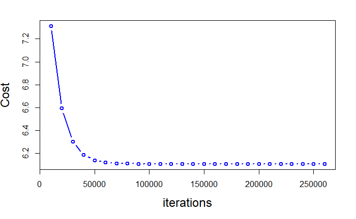
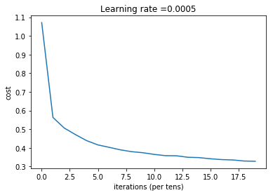
    # plot the cost
    plt.plot(np.squeeze(costs))
    plt.ylabel('cost')
    plt.xlabel('iterations (per tens)')
    plt.title("Learning rate =" + str(learning_rate))
    plt.show()
    
    return parameters

Now let us design the number of layers an neurons we need for our model. The size of the input is 12288(flattened pixel size for each image) and size of output layer is 1. We can decide on any number of input layers by adding more values in between. The number in between decides the number of neurons in that layer.

In [ ]:

### CONSTANTS ###
layers_dims = [12288, 20, 7,5, 1] #  5-layer model, 3 hidden layers, 1 input and 1 output layer

Let us run the model on our training dataset.

In [89]:

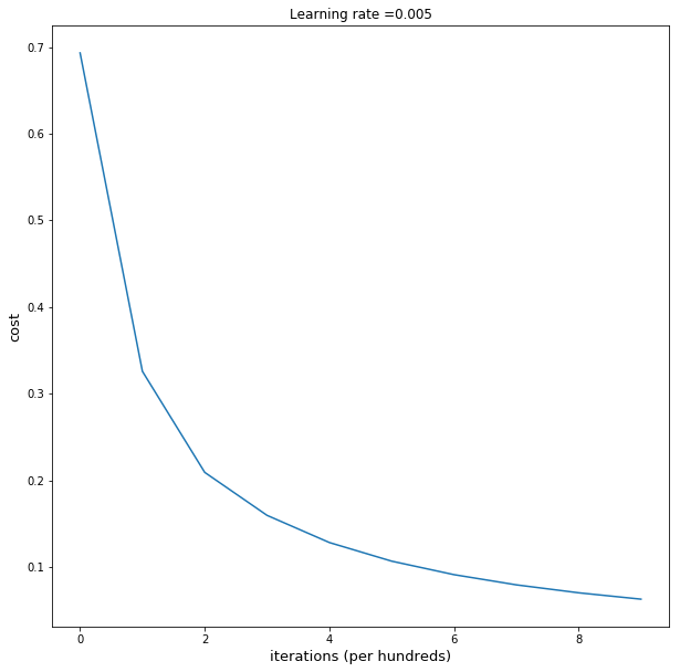
parameters = L_layer_model(train_x, y_train, layers_dims,learning_rate = 0.0005, num_iterations = 2000, print_cost = True)

Cost after iteration 0: 1.070965
Cost after iteration 100: 0.562904
Cost after iteration 200: 0.506057
Cost after iteration 300: 0.471016
Cost after iteration 400: 0.438274
Cost after iteration 500: 0.415518
Cost after iteration 600: 0.402530
Cost after iteration 700: 0.389101
Cost after iteration 800: 0.379235
Cost after iteration 900: 0.373636
Cost after iteration 1000: 0.364686
Cost after iteration 1100: 0.357966
Cost after iteration 1200: 0.357162
Cost after iteration 1300: 0.349248
Cost after iteration 1400: 0.347425
Cost after iteration 1500: 0.341249
Cost after iteration 1600: 0.336788
Cost after iteration 1700: 0.334838
Cost after iteration 1800: 0.329172
Cost after iteration 1900: 0.327770

Now let’s define a predict function which will use the trained model parameters to predict the gender of input images. Probabilities above or equal to 0.5 are considered as females and probabilities below 0.5 are considered as males.

In [96]:

def predict(X, y, parameters):
    """
    This function is used to predict the results of a  L-layer neural network.
    
    Arguments:
    X -- data set of examples you would like to label
    parameters -- parameters of the trained model
    
    Returns:
    p -- predictions for the given dataset X
    """
    
    m = X.shape[1]
    n = len(parameters) // 2 # number of layers in the neural network
    p = np.zeros((1,m))
    
    # Forward propagation
    probas, caches = L_model_forward(X, parameters)

    # convert probas to 0/1 predictions
    p=np.round(probas)
    
    #print results
    #print ("predictions: " + str(p))
    #print ("true labels: " + str(y))
    print("Accuracy: "  + str(np.sum((p == y)/m)))
        
    return p

Let’s check the accuracy of the algorithm on training and testing data.

In [101]:

print("Train Accuracy")
pred_train = predict(train_x, y_train, parameters)
print("Test Accuracy")
pred_test = predict(test_x, y_test, parameters)

Train Accuracy
Accuracy: 0.975
Test Accuracy
Accuracy: 0.75

With a single neuron, we got test accuracy of 65%. With a multilayered model, we improved our accurcy to 75%. Not bad!

Now let us define a function to look at the misclassified images.

In [94]:

def print_mislabeled_images(classes, X, y, p):
    """
    Plots images where predictions and truth were different.
    X -- dataset
    y -- true labels
    p -- predictions
    """
    a = p + y
    mislabeled_indices = np.asarray(np.where(a == 1))
    plt.rcParams['figure.figsize'] = (40.0, 40.0) # set default size of plots
    num_images = len(mislabeled_indices[0])
    for i in range(num_images):
        index = mislabeled_indices[1][i]
        
        plt.subplot(2, num_images, i + 1)
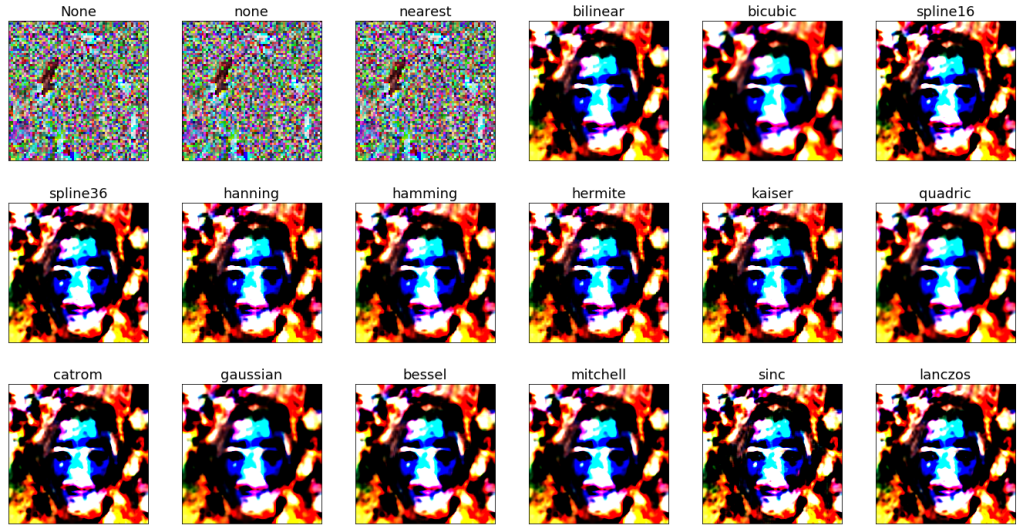
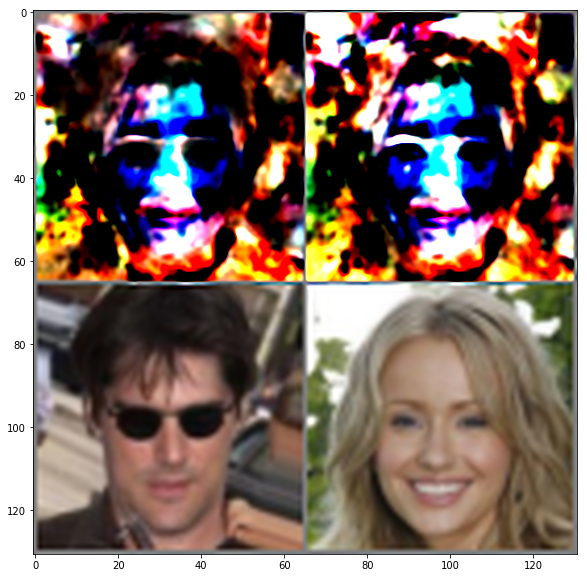
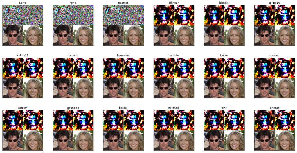
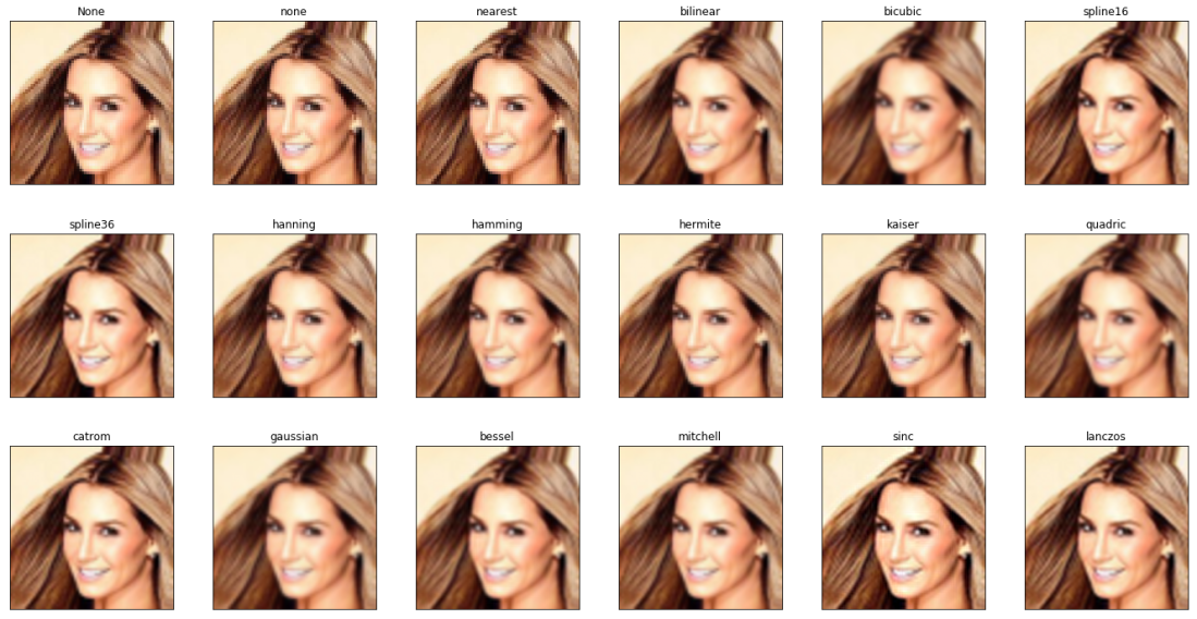
        plt.imshow(X[:,index].reshape(64,64,3), interpolation='sinc')
        plt.axis('off')
        plt.rc('font', size=20)
        plt.title("Prediction: " + classes[int(p[0,index])] + " \n Class: " + classes[y[0,index]])

In [95]:

print_mislabeled_images(classes, test_x, y_test, pred_test)

One of the biggest question now is can we improve the accuracy of the model. We probably can improve a bit more by further tuning the learning rate, number of layers and neurons and even trying out different kinds of activation functions. As you know by now, there are a lot of hyoerparameters which has to be tuned for the neural networks. That is one of the reason why it is very difficult to train a multi layered neural network or deeplearning model.

One other thing we notice is, there is a big difference between training accuracy and testing accuracy. This is probably a sign of overfitting. There are different ways of reducing overfitting, like regularization and dropout. I will discuss that in the next article.

–Jobil Louis Joseph

References: ‘Neural Networks and Deep Learning’ on Coursera by Andrew Ng
Calculus by Gilbert Strang

Image Processing and Neural Networks Intuition: Part 2

In the previous post, I talked about how to preprocess and explore image dataset. In this post, I will talk about how to model image data with neural networks having a single neuron, using sigmoid function. This is equivalent to logistic regression. Only difference is the way we estimate weights(coeffcients) of the the inputs. The traditional way of estimating logistic regression weights(coefficients) is to use analytical methods(an optimization technique). But the neural network way of estimating weights(coefficients) is to use gradient descent algorithm. To know more about different kinds of optimization techniques, you can check one of my previous post.

Before jumping to modeling, I will try to give an intuition about the sigmoid function.

 

Sigmoid function intuition

The sigmoid function is given by the formula,

For any input x, a(sigmoid of x) will vary between 0 and 1. When x is positive and large, e^x(numerator) and 1+e^x(denominator) will be approximately same and value of a will be one. Similarly when x is a large negative number, e^x will be approximately zero and value of a will be zero. Let’s see two examples.

import numpy as np 
x=500
print(1/(1+np.exp(-x)))

1.0

In [57]:

x=-500
print(1/(1+np.exp(-x)))

 Out[57}:

7.12457640674e-218

Another important aspect of sigmoid function is that it is a non-linear function in x. This fact becomes more powerful in case of multi layered neural networks, as it will help in unlocking many hidden non-linear patterns in the data. A single sigmoid function looks like the following graph, for different values of x.

In [114]:

import matplotlib.pyplot as plt 
%matplotlib inline

def sigmoid(z): 
  s = 1/(1+np.exp(-z)) 
  return s

x=np.linspace(-10,10,100)         #linspace generates 100 uniformly spaced values between -10 and 10
plt.figure(figsize=(10, 5))       #Setting up the figure size of width 10 and height 5
plt.plot(x,sigmoid(x),'b')        #Plot sigmoid(x) in Y-axis and x in X-axis with line color blue
plt.grid()                        #Add grid to the plot 
plt.rc('axes', labelsize=13)      #Set x label abd y label fontsize to 13
plt.xlabel('x')                   #Label x-axis 
plt.ylabel('a (sigmoid(x))')      #Label y axis
plt.rc('font', size=15)           #Set text fontsize default as 15
plt.suptitle('Sigmoid Function')  #Create a supertitle for the plot. You can use title as well

Out[114]:

 

As you can see from the graph, a(sigmoid(x)) varies between 0 and 1. This makes sigmoid function and in turn logistic regression suitable for binomial classification problem. That means we can use logistic regression or sigmoid function when the target varible has only two values(0 or 1). This makes it suitable for our purpose, in which we are trying to predict the gender of the celebrity from images. Gender(our target variable) has only two values in our dataset, male(0) and female(1).

Sigmoid function essentially gives out the probabilty target variable being 1 for a given input. i.e in our case given an image, sigmoid function gives the probability of that image being that of a female celebrity, since in our target variable female gender is indicated as 1. Although, probabilty of an image being male can be easily calculated as 1-sigmoid(input image) will give that.

Another point to remember is that, for our problem input x is a combination of variables or pixels to be precise. Let’s denote this combination of input variables as z.

where,
w1 = weight of the first variable (in our case the first pixel)
x1 = first variable (in our case, first pixel) and so on..
b = bias (similar to intercept in linear regression)

where  is the sigmoid function
and a is the predicted values(probabilities)
In matrix notation, the equations can be written as,

where ‘.’ indicates matrix multiplication
W is the row vector of all weights of dimension[1,num_px] num_px is the number of pixels(variables)
X is the input matrix of dimension[num_px,m] m = no.of training examples
A is the array of predicted values of dimension[1,m]

Cost Function

The unknowns in the above equations are weights(w’s) and bias(b). The idea of logistic regression or single neuron neural network(from now on I will use this terminology) is to find the best values of weights and bias which gives the minimum error(cost).

So for training the model first we have to define the cost function. We define the cost function for the binomial prediction as

where,
J(a,y) is the cost which is a function of a and y and it is a scalar meaning single value. This cost is called negative log likelihood. Lower the cost, better the model
m = number of training examples
y = array of true labels or actual values
a =  , the predicted values
z = w1x1 + w2x2 +…+w_n*x_n + b

In matrix form we write it as,

where,
m is the number of training examples
 is the transpose of A which is the array of predicted values of dimensions [m,1]
Y is the array actual values or true labels of dimensions [1,m]

Steps to train a single neuron

Now we have to use gradient descent to find the values of W and b that minimizes the cost. For an intuitive and detailed explanation of gradient descent, you can check the post which I mentioned earlier.

In short, training of single neuron neural network using gradient descent involves the following steps:

1) Initialize parameters i.e W and b

2) Forward Propagation: Calculate Z and A using the initialized parameters

3) Compute cost

4) Backward propagation: Take gradient(derivative) of cost function with respect to W and b

5) Use the gradients to update the values of W and b

6) Repeat steps 2 to 5 for a fixed number of times

Forward Propagation

In steps 2 and 3, we calculate the values of A and Z as mentioned before and compute the cost. This step is called forward propagation.

dZ =  = A-Y

dW =  = 

db =  = 

where  is the transpose of X.

 

In the above diagram, backward propagation is highlighted by red colored line. From the point of view of logical flow of the network, backward propagation starts from the cost and reaches W. The intuition is we need to update the parameters(W and b) of the model to minimze cost, and in order to do that we need to find the derivative of cost w.r.t the parameters we want to update. However, cost is not directly dependent on parameter(W and b) but on functions(A and Z) which uses these parameters. Hence we need to use chain rule to calculate the derivative of cost w.r.t to parameters. Each derivative term in the chain rule happens at a different part in the model, which starts at cost and flows backward.

For detailed explanation and derivations you can refer this post.

Parameter Updates

In step 5, we need to update the parameters as follows

Here  is a parameter called learning rate. It controls how big the update(or step) is in each iteration. If  is too small, it may take a long time to find the best parameters and if  is too big we may overshoot and never reach the optimal parameters.

 

In step 6, we need to repeat the steps a fixed number of times. There is no rule as such how many iterations we have to run. It varies from dataset to dataset. If we set alpha to a very small value, we may need to iterate more number of times. Generally it’s a hyperparameter which we have to tune.

That’s all we need to know to implement a single neuron neural network.

So to reiterate the steps involved:

1) Initialize parameters i.e W and b

2) Forward Propagation: Calculate Z and A using the initialized parameters

3) Compute cost

4) Backward propagation: Take gradient(derivative) of cost function with respect to W and b

5) Use the gradients to update the values of W and b

6) Repeat steps 2 to 5 for a fixed number of times

Single Neuron Implementation

I will continue from where I stopped in the last article. I will continue with the same problem and same dataset.

Our problem statement was to predict the gender of the celebrity from the image.

After preprocessing, our final data sets were train_x(train data input) , y_train(target variable for the training set), test_x(test data input) , y_test(target variable for the testing set).

Loading the necessary libraries

In [124]:

import os
import numpy as np
from scipy.misc import imresize
import matplotlib.pyplot as plt
%matplotlib inline

Let’s take a quick look at the data attributes.

In [128]:

m_train = train_x.shape[1]
m_test = y_test.shape[1]
num_px = train_x_orig.shape[1]


print ("Number of training examples: m_train = " + str(m_train))
print ("Number of testing examples: m_test = " + str(m_test))
print ("Height/Width of each image: num_px = " + str(num_px))
print ("Each image is of size: (" + str(num_px) + ", " + str(num_px) + ", 3)")
print ("train_x shape: " + str(train_x.shape))
print ("y_train shape: " + str(y_train.shape))
print ("test_x shape: " + str(test_x.shape))
print ("y_test shape: " + str(y_test.shape))

 Out[128]:

Number of training examples: m_train = 80
Number of testing examples: m_test = 20
Height/Width of each image: num_px = 64
Each image is of size: (64, 64, 3)
train_x shape: (12288, 80)
y_train shape: (1, 80)
test_x shape: (12288, 20)
y_test shape: (1, 20)

Step 1) Initialize parameters i.e W and b 

Let’s write a function to initialize W and b. There are different intialization techniques. For this exercise, we will intialize both W and b to zero.

In [131]:

def initialize_with_zeros(dim):
    #Function takes in a parameter dim whic is equal to no of columns or pixels in the dataset
    w = np.zeros((1,dim))
    b = 0
    assert(w.shape == (1, dim)) #Assert statement ensures W and b has the required shape
    assert(isinstance(b, float) or isinstance(b, int))
    return w, b

Steps 2, 3 and 4 Forward Propagation, Cost computation and Backward propagation 

We will define a sigmoid function first, which will take any array or vector as an input and returns the sigmoid of the input.

In [130]:

def sigmoid(z):
    s = 1/(1+np.exp(-z))   
    return s

Now let’s write a function called propagate, which will take W(weights),b(bias),X(input matrix) and Y(target variable) as inputs. It should return cost and gradients dW and db.
We need to calculate the following:

A= = 

Cost = 

dW =  = 

db =  = 

where ‘.’ indicates matrix multiplication. In python, np.dot(numpy.dot) function is used for matrix multiplication.

In [129]:

def propagate(w, b, X, Y):
    """
    Arguments:
    w -- weights, a numpy array of size (num_px * num_px * 3, 1)
    b -- bias, a scalar
    X -- data of size (num_px * num_px * 3, number of examples)
    Y -- true "label" vector (containing 0 if male celebrity, 1 if female celebrity) of size (1, number of examples)

    Return:
    cost -- negative log-likelihood cost for logistic regression
    dw -- gradient of the loss with respect to w, thus same shape as w
    db -- gradient of the loss with respect to b, thus same shape as b
    
    """
    
    m = X.shape[1]
    
    # FORWARD PROPAGATION (FROM X TO COST)
    A = sigmoid(np.dot(w,X)+b)                                    # compute sigmoid- np.dot is used for matrix multiplication
    cost = (-1/m)*(np.dot(Y,np.log(A.T))+ np.dot((1-Y),np.log((1-A).T)))                                 # compute cost
    
    # BACKWARD PROPAGATION (TO FIND GRAD)
    dw = (1/m)*np.dot((A-Y),X.T)
    db = (1/m)*np.sum((A-Y))

    assert(dw.shape == w.shape)
    assert(db.dtype == float)
    cost = np.squeeze(cost)                                      #to make cost a scalar i.e a single value
    assert(cost.shape == ())
    
    grads = {"dw": dw,
             "db": db}
    
    return grads, cost

Steps 5 and 6 Optimization:Update parameters and iterate 

Let’s define a function optimize which will repeat steps 2 through 5 for a given number of times.

Steps 2 till 4 can be calculated by calling the propagate function. We need to define step 5 here. i.e parameter updates. Update rules are:

were  is the learning rate.

After iterating through the given number of iterations, this function should return the final weights and bias

In [162]:

def optimize(w, b, X, Y, num_iterations, learning_rate, print_cost = False):
    """
    This function optimizes w and b by running a gradient descent algorithm
    
    Arguments:
    w -- weights, a numpy array of size (num_px * num_px * 3, 1)
    b -- bias, a scalar
    X -- data of shape (num_px * num_px * 3, number of examples)
    Y -- true "label" vector (containing 0 if male celebrity, 1 if female celebrity) of size (1, number of examples)
    num_iterations -- number of iterations of the optimization loop
    learning_rate -- learning rate of the gradient descent update rule
    print_cost -- True to print the loss every 100 steps
    
    Returns:
    params -- dictionary containing the weights w and bias b
    grads -- dictionary containing the gradients of the weights and bias with respect to the cost function
    costs -- list of all the costs computed during the optimization, this will be used to plot the learning curve.
    
    """
    
    costs = []
    
    for i in range(num_iterations):           #This will iterate i from 0 till num_iterations-1
        
        
        # Cost and gradient calculation
        grads, cost = propagate(w, b, X, Y)
        
        # Retrieve derivatives from grads
        dw = grads["dw"]
        db = grads["db"]
        
        # update rule 
        w = w-learning_rate*dw
        b = b-learning_rate*db
        
        # Record the costs for every 100th iteration
        if i % 100 == 0:
            costs.append(cost)
        
        # Print the cost every 100 training examples
        if print_cost and i % 100 == 0:
            print ("Cost after iteration %i: %f" %(i, cost))
    
        # plot the cost
    plt.rcParams['figure.figsize'] = (10.0, 10.0)    
    plt.plot(np.squeeze(costs))
    plt.ylabel('cost')
    plt.xlabel('iterations (per hundreds)')
    plt.title("Learning rate =" + str(learning_rate))
    plt.show()
    params = {"w": w,
              "b": b}
    
    grads = {"dw": dw,
             "db": db}
    
    return params, grads, costs

Prediction using learned parameters

From the previous function we will get the final weights and bias. We can use those weights to predict the target variable(gender) on new data(test data). Let’s define a function for prediction capability. If the predicted probability is 0.5 or less, the image will be calssified as 0(male) else 1(female).

In [136]:

def predict(w, b, X):
    '''
    Predict whether the label is 0 or 1 using learned logistic regression parameters (w, b)
    
    Arguments:
    w -- weights, a numpy array of size (num_px * num_px * 3, 1)
    b -- bias, a scalar
    X -- data of size (num_px * num_px * 3, number of examples)
    
    Returns:
    Y_prediction -- a numpy array (vector) containing all predictions (0/1) for the examples in X
    '''
    
    m = X.shape[1]
    Y_prediction = np.zeros((1,m))
    #w = w.reshape(X.shape[0], 1)
    
    # Compute vector "A" predicting the probabilities of having a female celebrity in the picture
    A = sigmoid(np.dot(w,X)+b)   
    Y_prediction=np.round(A)

    assert(Y_prediction.shape == (1, m))
    
    return Y_prediction

Putting everything together

Let’s put training and prediction into a sigle function called model, which will train the model on training data and predict on testing data and return accuracy of the model. Since we have to predict 0 or 1, we can calculate accuray using the formula:

It indicates what percentage of images have been rightly classified or predicted.
You can define any accuracy or evaluation metrics. However, in this series we will use accuracy defined as above.

In [139]:

def model(X_train, Y_train, X_test, Y_test, num_iterations = 2000, learning_rate = 0.5, print_cost = False):
    """
    Builds the logistic regression model by calling the function implemented previously
    
    Arguments:
    X_train -- training set represented by a numpy array of shape (num_px * num_px * 3, m_train)
    Y_train -- training labels represented by a numpy array (vector) of shape (1, m_train)
    X_test -- test set represented by a numpy array of shape (num_px * num_px * 3, m_test)
    Y_test -- test labels represented by a numpy array (vector) of shape (1, m_test)
    num_iterations -- hyperparameter representing the number of iterations to optimize the parameters
    learning_rate -- hyperparameter representing the learning rate used in the update rule of optimize()
    print_cost -- Set to true to print the cost every 100 iterations
    
    Returns:
    d -- dictionary containing information about the model.
    """
    
    # initialize parameters with zeros
    m_train=X_train.shape[0]
    w, b = initialize_with_zeros(m_train)

    # Gradient descent
    parameters, grads, costs = optimize(w, b, X_train, Y_train, num_iterations= num_iterations, learning_rate = learning_rate, print_cost = print_cost)
    
    # Retrieve parameters w and b from dictionary "parameters"
    w = parameters["w"]
    b = parameters["b"]
    
    # Predict test/train set examples
    Y_prediction_test = predict(w, b, X_test)
    Y_prediction_train = predict(w, b, X_train)

    # Print train/test Errors
    print("train accuracy: {} %".format(100*(1 - np.mean(np.abs(Y_prediction_train - Y_train)) )))
    print("test accuracy: {} %".format(100*(1 - np.mean(np.abs(Y_prediction_test - Y_test)) )))

    
    d = {"costs": costs,
         "Y_prediction_test": Y_prediction_test, 
         "Y_prediction_train" : Y_prediction_train, 
         "w" : w, 
         "b" : b,
         "learning_rate" : learning_rate,
         "num_iterations": num_iterations}
    
    return d

In [167]:

d = model(train_x, y_train, test_x, y_test, num_iterations = 1000, learning_rate = 0.005, print_cost = True)

 Out[167]:

Cost after iteration 0: 0.693147
Cost after iteration 100: 0.325803
Cost after iteration 200: 0.209219
Cost after iteration 300: 0.159637
Cost after iteration 400: 0.128275
Cost after iteration 500: 0.106781
Cost after iteration 600: 0.091209
Cost after iteration 700: 0.079450
Cost after iteration 800: 0.070282
Cost after iteration 900: 0.062948

train accuracy: 100.0 %
test accuracy: 65.0 %

The accuracy of the model is around 65% with learning rate =0.005 and number of iterations =1000. Probably we can achieve bit more better results by tuning these two parameters.

Now, let’s take a look at the mis labeled or wrongly predicted images.

In [168]:

def print_mislabeled_images(classes, X, y, p):
    """
    Plots images where predictions and truth were different.
    X -- dataset
    y -- true labels
    p -- predictions
    """
    a = p + y
    mislabeled_indices = np.asarray(np.where(a == 1))
    plt.rcParams['figure.figsize'] = (40.0, 40.0) # set default size of plots
    num_images = len(mislabeled_indices[0])
    for i in range(num_images):
        index = mislabeled_indices[1][i]
        
        plt.subplot(2, num_images, i + 1)
        plt.imshow(X[:,index].reshape(64,64,3), interpolation='sinc')
        plt.axis('off')
        plt.rc('font', size=20)
        plt.title("Prediction: " + classes[int(p[0,index])] + " \n Class: " + classes[y[0,index]])

In [170]:

print_mislabeled_images(classes, test_x, y_test, d["Y_prediction_test"])

So now we have completed training a single node neural network. We have achieved an accuracy of 65 %. Not bad for a single neuron or simple logistic regression. It’s a bit long post but understanding the basics is the key to understand more complex algorithms. Sigmoid function(or similar functions) is the building block for Neural Networks, Deep learning and AI. I hope this article gave a good intuition about the sigmoid function and neural network approach.

Building on top of this article, in the next post, I will talk about how to train a multi layer neural network.

Before wrapping up, I will try to show what the neuron has learned at the end of training. Now this part is not for weak hearted people. Continue only if you are brave and curious :D.Let’s use the final weights to multiply corresponding pixels in training data and scale by a factor 255, since we divided pixels by 255 for standardization.

Now let’s plot an image from the reconstructed data.

In [237]:

test=d["w"].T*train_x*255
test=test.T.reshape(80,64,64,3)
plt.rcParams['figure.figsize'] = (10.0, 10.0)
plt.imshow(test[0], interpolation='sinc')

Out[237]:

<matplotlib.image.AxesImage at 0x25f903a3b70>

You may either find the image artistic or scary or weird. Neverthless it’s still very interesting, atleast for me ;). For plotting the above image I used sinc interpolation. We can try different interpolations and see the effects.

In [238]:

methods = [None, 'none', 'nearest', 'bilinear', 'bicubic', 'spline16',
           'spline36', 'hanning', 'hamming', 'hermite', 'kaiser', 'quadric',
           'catrom', 'gaussian', 'bessel', 'mitchell', 'sinc', 'lanczos']

# Fixing random state for reproducibility
np.random.seed(19680801)


fig, axes = plt.subplots(3, 6, figsize=(24, 12),
                         subplot_kw={'xticks': [], 'yticks': []})

fig.subplots_adjust(hspace=0.3, wspace=0.05)

for ax, interp_method in zip(axes.flat, methods):
    ax.imshow(test[0], interpolation=interp_method, cmap=None)
    ax.set_title(interp_method)

plt.show()

 

 

Let’s create a montage and compare the reconstructed images vs original.

In [239]:

def montage(images, saveto='montage.png'):
    """Draw all images as a montage separated by 1 pixel borders.
    Also saves the file to the destination specified by `saveto`.
    Parameters
    ----------
    images : numpy.ndarray
        Input array to create montage of.  Array should be:
        batch x height x width x channels.
    saveto : str
        Location to save the resulting montage image.
    Returns
    -------
    m : numpy.ndarray
        Montage image.
    """
    if isinstance(images, list):
        images = np.array(images)
    img_h = images.shape[1]
    img_w = images.shape[2]
    n_plots = int(np.ceil(np.sqrt(images.shape[0])))
    if len(images.shape) == 4 and images.shape[3] == 3:
        m = np.ones(
            (images.shape[1] * n_plots + n_plots + 1,
             images.shape[2] * n_plots + n_plots + 1, 3)) * 0.5
    else:
        m = np.ones(
            (images.shape[1] * n_plots + n_plots + 1,
             images.shape[2] * n_plots + n_plots + 1)) * 0.5
    for i in range(n_plots):
        for j in range(n_plots):
            this_filter = i * n_plots + j
            if this_filter < images.shape[0]:
                this_img = images[this_filter]
                m[1 + i + i * img_h:1 + i + (i + 1) * img_h,
                  1 + j + j * img_w:1 + j + (j + 1) * img_w] = this_img
    #plt.imsave(arr=m, fname=saveto)
    return m

The above function can be used to create montages. Now let’s combine some of the reconstructed images and original data and create a montage.

In [240]:

compare = np.concatenate((test[52:54], data[52:54]), axis=0)
compare.shape

Out[240]:

(4, 64, 64, 3)

Now let us try to create the montage with two different interpolations.

In [241]:

plt.imshow(montage(compare,saveto='montage.png'),interpolation='spline36')
plt.show()
plt.imshow(montage(compare,saveto='montage.png'),interpolation='bicubic')
plt.show()

If you look carefully, in the reconstructed image, hair colors of the image have been captured differently. This is an indication that the algorithm has learned some of the facial features from the data.

Also, other thing we can do is to generate the montage with different interpolations for comparison.

In [232]:

methods = [None, 'none', 'nearest', 'bilinear', 'bicubic', 'spline16',
           'spline36', 'hanning', 'hamming', 'hermite', 'kaiser', 'quadric',
           'catrom', 'gaussian', 'bessel', 'mitchell', 'sinc', 'lanczos']

# Fixing random state for reproducibility
np.random.seed(19680801)


fig, axes = plt.subplots(3, 6, figsize=(24, 12),
                         subplot_kw={'xticks': [], 'yticks': []})

fig.subplots_adjust(hspace=0.3, wspace=0.05)

for ax, interp_method in zip(axes.flat, methods):
    ax.imshow(montage(compare,saveto='montage.png'), interpolation=interp_method, cmap=None)
    ax.set_title(interp_method)

plt.show()

 

 

Images are very interesting. We can find very interesting patterns and visulaize how an algorithm learns to identify patterns in the image. It always amazes me. On that note I am putting my pen down on this article. In the next article, I will talk about multi layer neural networks and try to explore what the neurons have learned from the images.

 

Jobil Louis Joseph

References:
‘Neural Networks and Deep Learning’ on Coursera by Andrew Ng
Calculus by Gilbert Strang

Image Processing and Neural Networks Intuition: Part 1

In this series, I will talk about training a simple neural network on image data. To give a brief overview, neural networks is a kind of supervised learning. By this I mean, the model needs to train on historical data to understand the relationship between input variables and target variables. Once trained, the model can be used to predict target variable on new input data. In the previous posts, we have written about linear, lasso and ridge regression. All those methods come under supervised learning. But what is special about neural networks is, it works really well for image, audio, video and language datasets. A multilayer neural network and its variations are commonly called deep learning.

In this blog, I will focus on handling and processing the image data. In the next blog, I will show how to train the model. I will use python for implementation as python as many useful functions for image processing.  If you are new to python, I recommend you to quickly take a numpy (till array manipulation) and matplotlib tutorial.

Main contents of this article:

a) Exploring image dataset: Reading images, printing image arrays and actual images, decomposing images into different color channels

b) Cropping and Resizing images: Cropping rectangle images to a square, resizing high resolution images to a lower resolution for easier processing, creating gray scale images from color images and standardizing image data

c) Colormapping and Interpolation: Converting no color channel images to color images using different themes. Interpolating after resizing or reducing resolution of images to for retaining quality and information.

d) Montage Creation and Preparing image data for modeling

Okay! Let’s get started. First let’s get some data set. This data is shared in the course on kadanze about Creative Applications of Deeplearning by Parag Mital. This data contains pictures of celebrities. Original source can be found here along with some description http://mmlab.ie.cuhk.edu.hk/projects/CelebA.html.

In the original dataset, there are around 200,000 pictures. For the purpose of this blog, we will use 100 images. The following code will download 100 images.

# Load the os library
import os

# Load the request module
import urllib.request

if not os.path.exists('img_align_celeba'):
    
    # Create a directory
    os.mkdir('img_align_celeba')

    # Now perform the following 100 times:
    for img_i in range(1, 101):

        # create a string using the current loop counter
        f = '000%03d.jpg' % img_i

        # and get the url with that string appended the end
        url = 'https://s3.amazonaws.com/cadl/celeb-align/' + f

        # We'll print this out to the console so we can see how far we've gone
        print(url, end='\r')

        # And now download the url to a location inside our new directory
        urllib.request.urlretrieve(url, os.path.join('img_align_celeba', f))
else:
    print('Celeb Net dataset already downloaded')

If the dataset is not downloaded, the above code will download it. Let’s read the downloaded images into a variable.

files = [os.path.join('img_align_celeba', file_i)
 for file_i in os.listdir('img_align_celeba')
 if '.jpg' in file_i]

Let’s add a target column. Here we will try to identify whether a picture shows a male celebrity or female celebrity. Value 1 denotes ‘Female celebrity’ and 0 denotes ‘male celebrity’.

y=np.array([1,1,0,1,1,1,0,0,1,1,1,0,0,1,0,0,1,1,1,0,0,1,0,1,0,1,1,1,1,0,1,0,0,1,1,0,0,0,1,1,0,1,1,1,1,1,1,0,0,0,0,0,0,1,0,0,1,1,1,0,0,1,1,0,0,1,0,0,0,0,1,0,1,1,1,0,1,1,0,0,0,0,1,1,1,1,1,1,1,0,0,1,1,1,1,1,1,1,1,1])
y=y.reshape(1,y.shape[0])
classes=np.array(['Male', 'Female'])

y_train=y[:,:80]
y_test=y[:,80:]

Now let’s take a closer look at our data set. For this, we will use the matplotlib library for plotting. We can also use it to view the images in our data.

import matplotlib.pyplot as plt
%matplotlib inline

Exploring image dataset

In this section, we will try to understand our image data better. Let’s plot an image from the data set(in this case the first image)

plt.imread(files[0])

Output:

array([[[253, 231, 194],
        [253, 231, 194],
        [253, 231, 194],
        ..., 
        [247, 226, 225],
        [254, 238, 222],
        [254, 238, 222]],

       [[253, 231, 194],
        [253, 231, 194],
        [253, 231, 194],
        ..., 
        [249, 228, 225],
        [254, 238, 222],
        [254, 238, 222]],

       [[253, 231, 194],
        [253, 231, 194],
        [253, 231, 194],
        ..., 
        [250, 231, 227],
        [255, 239, 223],
        [255, 239, 223]],

       ..., 
       [[140,  74,  26],
        [116,  48,   1],
        [146,  78,  33],
        ..., 
        [122,  55,  28],
        [122,  56,  30],
        [122,  56,  30]],

       [[130,  62,  15],
        [138,  70,  23],
        [166,  98,  53],
        ..., 
        [118,  49,  20],
        [118,  51,  24],
        [118,  51,  24]],

       [[168, 100,  53],
        [204, 136,  89],
        [245, 177, 132],
        ..., 
        [118,  49,  20],
        [120,  50,  24],
        [120,  50,  24]]], dtype=uint8)

It prints some numbers. Here each tuple (the innermost array) represents a pixel. As you can see, it has 3 values, one corresponding to each color channel, RGB (Red, Green Blue). To view the data as image, we have to use ‘imshow’ function

img = plt.imread(files[0])
plt.imshow(img)

 Output:

 

Let’s see the shape(dimensions) of the image

img.shape

Output:

(218, 178, 3)

This means height of the image is 218 pixels,width 178 pixels and each pixel has 3 color channels(RGB). We can view the image using each of the color channels.

plt.figure()
plt.imshow(img[:, :, 0])
plt.figure()
plt.imshow(img[:, :, 1])
plt.figure()
plt.imshow(img[:, :, 2])

Output:

Cropping and resizing images

For many of the deeplearning and image processing applications, we will need to crop the image to a square and resize it for faster processing. The following function will crop any rectangle image(height != width) to a square image

def imcrop_tosquare(img):
    if img.shape[0] > img.shape[1]:
        extra = (img.shape[0] - img.shape[1]) // 2
        crop = img[extra:-extra, :]
    elif img.shape[1] > img.shape[0]:
        extra = (img.shape[1] - img.shape[0]) // 2
        crop = img[:, extra:-extra]
    else:
        crop = img
    return crop

Now we will resize the image to 64 by 64 pixels(height=64,width=64). For resizing, we can use the imresize function from scipy.

from scipy.misc import imresize

square = imcrop_tosquare(img)
rsz = imresize(square, (64, 64))
plt.imshow(rsz)
print(rsz.shape)

Output:

(64, 64,3)

 

As we can see from the shape of the image, it has been resized to (64,64,3). If we take the mean of each color channels(RGB), we will get a grayscale image.

mean_img = np.mean(rsz, axis=2)
print(mean_img.shape)
plt.imshow(mean_img, cmap='gray')

Output:

(64, 64)

Colormapping and interpolating images

When there is no color channel for an image, you can use different availble color maps provided by matplotlib. Following code iterates through different color maps for the above image(with no color channel) and plots it. For your purposes, you can choose the best one if you come across such images. It is also an easy way to convert grayscale images to color.

mean_img = np.mean(rsz, axis=2)
methods = [None,'viridis', 'plasma', 'inferno', 'magma','Greys', 'Purples', 'Blues', 'Greens', 'Oranges', 'Reds',
 'YlOrBr', 'YlOrRd', 'OrRd', 'PuRd', 'RdPu', 'BuPu','GnBu', 'PuBu', 'YlGnBu', 'PuBuGn', 'BuGn', 'YlGn',
 'binary', 'gist_yarg', 'gist_gray', 'gray', 'bone', 'pink', 'spring', 'summer', 'autumn', 'winter', 'cool', 'Wistia',
 'hot', 'afmhot', 'gist_heat', 'copper','PiYG', 'PRGn', 'BrBG', 'PuOr', 'RdGy', 'RdBu','RdYlBu', 'RdYlGn', 
 'Spectral', 'coolwarm', 'bwr', 'seismic','Pastel1', 'Pastel2', 'Paired', 'Accent','Dark2', 'Set1', 'Set2', 'Set3',
 'tab10', 'tab20', 'tab20b', 'tab20c','flag', 'prism', 'ocean', 'gist_earth', 'terrain', 'gist_stern','gnuplot', 
 'gnuplot2', 'CMRmap', 'cubehelix', 'brg', 'hsv','gist_rainbow', 'rainbow', 'jet', 'nipy_spectral', 'gist_ncar']

np.random.seed(19680801)
fig, axes = plt.subplots(10, 8, figsize=(16, 32),
 subplot_kw={'xticks': [], 'yticks': []})

fig.subplots_adjust(hspace=0.3, wspace=0.05)

for ax, interp_method in zip(axes.flat, methods):
 ax.imshow(mean_img, interpolation='sinc',cmap=interp_method)
 ax.set_title(interp_method)
plt.show()

Output:

 

Now let’s crop all the rectangle images as square and resize all the images in the dataset to size 64, 64, 3.

imgs = []
for file_i in files:
    img = plt.imread(file_i)
    square = imcrop_tosquare(img)
    rsz = imresize(square, (64, 64))
    imgs.append(rsz)
print(len(imgs))

Output:

100

Let’s combine all the images into a variable

data = np.array(imgs)

If you are familiar with machine learning, you will know the about data standardization. It means generally bringing down the range of an input variable. Same can be done with image data as well. However, for images there is an easy way to standardize. We can simply divide each of the values by 255, as each pixel can have values from 0-255. This will change the scale from 0-255 to 0-1. This will make sure while taking exponents in logistic regression, we won’t overflow the system.

data=data/255

plt.imshow(data[0])

Output:

 

When we reduce the resolution, we lose some information. We can use different kinds of interpolation to overcome this. The following code shows the effect of different kinds of interpolation. While plotting images after resizing, you can choose any interpolation you like.

data.shape
methods = [None, 'none', 'nearest', 'bilinear', 'bicubic', 'spline16',
 'spline36', 'hanning', 'hamming', 'hermite', 'kaiser', 'quadric',
 'catrom', 'gaussian', 'bessel', 'mitchell', 'sinc', 'lanczos']

np.random.seed(19680801)

fig, axes = plt.subplots(3, 6, figsize=(24, 12),
 subplot_kw={'xticks': [], 'yticks': []})

fig.subplots_adjust(hspace=0.3, wspace=0.05)

for ax, interp_method in zip(axes.flat, methods):
 ax.imshow(data[0], interpolation=interp_method, cmap=None)
 ax.set_title(interp_method)

plt.show()

Output:

 

Let’s see the shape(dimensions) of the variable data.

data.shape

Output:

(100, 64, 64, 3)

Shape of the data is 100,64,64,3. This means there are 100 images of size(64,64,3)

Montage creation

Till now we have been inspecting one image at a time. To view all images, we can use the following function to create a montage of all the images

def montage(images, saveto='montage.png'):
    """Draw all images as a montage separated by 1 pixel borders.
    Also saves the file to the destination specified by `saveto`.
    Parameters
    ----------
    images : numpy.ndarray
        Input array to create montage of.  Array should be:
        batch x height x width x channels.
    saveto : str
        Location to save the resulting montage image.
    Returns
    -------
    m : numpy.ndarray
        Montage image.
    """
    if isinstance(images, list):
        images = np.array(images)
    img_h = images.shape[1]
    img_w = images.shape[2]
    n_plots = int(np.ceil(np.sqrt(images.shape[0])))
    if len(images.shape) == 4 and images.shape[3] == 3:
        m = np.ones(
            (images.shape[1] * n_plots + n_plots + 1,
             images.shape[2] * n_plots + n_plots + 1, 3)) * 0.5
    else:
        m = np.ones(
            (images.shape[1] * n_plots + n_plots + 1,
             images.shape[2] * n_plots + n_plots + 1)) * 0.5
    for i in range(n_plots):
        for j in range(n_plots):
            this_filter = i * n_plots + j
            if this_filter < images.shape[0]:
                this_img = images[this_filter]
                m[1 + i + i * img_h:1 + i + (i + 1) * img_h,
                  1 + j + j * img_w:1 + j + (j + 1) * img_w] = this_img
    plt.imsave(arr=m, fname=saveto)
    return m

plt.figure(figsize=(10, 10))
plt.imshow(montage(imgs,saveto='montage.png').astype(np.uint8))

Output:

Data Preparation for modeling

Let’s split the data into train and test. Train data will be used to train the model. Then we will predict on test data to check the accuracy of the trained model.

train_x_orig=data[:80,:,:,:]
test_x_orig=data[80:,:,:,:]

Unlike regression model, logistic regression is used to predict a binomial variable.i.e means a variable which takes only two values. This suits perfectly for us as we are trying to predict from the images whether it is a male or female celebrity.

m_train = train_x_orig.shape[0]
m_test = y_test.shape[1]
num_px = train_x_orig.shape[1]


print ("Number of training examples: m_train = " + str(m_train))
print ("Number of testing examples: m_test = " + str(m_test))
print ("Height/Width of each image: num_px = " + str(num_px))
print ("Each image is of size: (" + str(num_px) + ", " + str(num_px) + ", 3)")
print ("train_x shape: " + str(train_x_orig.shape))
print ("y_train shape: " + str(y_train.shape))
print ("test_x shape: " + str(test_x_orig.shape))
print ("y_test shape: " + str(y_test.shape))

 Output:

Number of training examples: m_train = 80
Number of testing examples: m_test = 20
Height/Width of each image: num_px = 64
Each image is of size: (64, 64, 3)
train_x shape: (80, 64, 64, 3)
y_train shape: (1, 80)
test_x shape: (20, 64, 64, 3)
y_test shape: (1, 20)

For the purpose of training, we have to reshape our data or flatten our data. After flattening, the shape of our data should become (height * width * 3, number of examples). After flattening, every column will represent an image.

train_x = train_x_orig.reshape(train_x_orig.shape[0],-1).T
test_x = test_x_orig.reshape(test_x_orig.shape[0],-1).T

print ("train_x flatten shape: " + str(train_x.shape))
print ("test_x flatten shape: " + str(test_x.shape))

 Output:

train_x flatten shape: (12288, 80)
test_x flatten shape: (12288, 20)

Now we have our data set ready. In the next part, I will talk about how to train the model using simple logistic regression using gradient descent. Meanwhile, If you want to know more about gradient descent check it out here.

 

–Jobil Louis Joseph

 

References:

‘Creative Applications of Deep Learning with Tensorflow’ on Kadenze by Parag Mital ‘Neural Networks and Deep Learning’ on Coursera by Andrew Ng

Optimization techniques: Finding maxima and minima

In the last post, we talked about how to estimate the coefficients or weights of linear regression. We estimated weights which give the minimum error. Essentially it is an optimization problem where we have to find the minimum error(cost) and the corresponding coefficients. In a way, all supervised learning algorithms have optimization at the crux of it where we will have to find the model parameters which gives the minimum error(cost). In this post, I will explain some onf the most commonly used methods to find the maxima or minima of the cost function.

Before starting with the cost function(average((actual -predicted)^2)), I will talk about how to find the maxima or minima of a curve. Let’s consider a curve

y= x^2 + 5x             -eq(1)

Figure 1

Let’s say we want to find the minimum point in y and value of x which gives that minimum y. There are many ways to find this. I will explain three of those.

1) Search based methods: Here the idea is to search for the minimum value of y by feeding in different values of x. There are two different ways to do this.

a) Grid search: In grid search, you give a list of values for x(as in a grid) and calculate y and see the minimum of those.

b) Random search: In this method, you randomly generate values of x and compute y and find the minimum among those.

The drawback of search based methods is that there is no guarantee that we will find a local or global minimum. Global minimum means the overall minimum of a curve. Local minimum means a point which is minimum relatively to its neighboring values.

Figure 2

However, when a cost function depends on many parameters, search based methods are very useful to narrow down the search space. For example, if y was dependent on x1,x2,x3..xn, then search based methods will perform reasonably well.

2) Analytical: In analytical method, we find the point in the curve where the slope is 0. The slope of a curve is given by its derivative. Derivative of y, dy/dx, means how much y changes for a small change in x. It is same as the definition of slope. The slope is zero at the point in the curve where it is parallel to the x-axis (in the above figure all minima and maxima points have slope =0). The slope is zero for minima and maxima points. That means after finding the point where the slope is zero, we need to determine whether that point is a minima or maxima.

So in our equation 1, to find the minima of the curve, first, we need to find the point where the slope is zero. To do that we need to find the derivative of the curve and equate it to zero.

Before calculating derivative, a quick calculus refresher

 

For finding the slope of our curve, we need to find the derivative of our equation(1).

y= x^2 + 5x     

By summation rule,

y’ = (x^2)’ +(5x)’

==> y’ = slope of y = 2x+ 5    eq(2)

To find the point in the curve where the slope is zero, we need to equate the first derivative to zero and solve for x.

==> 2x+5=0

==> x= -5/2 = -2.5

Value of y when x = -2.5,

y= (-2.5 ^2) + 5*-2.5 = -6.25

Now we have found a point in the curve where the slope is zero. To determine whether it is a minima or maxima, we need to find the second derivative where y =0. From equation 2, y’= 2x+5. Again differentiating y’ w.r.t x,

y” = 2   eq(3)

y”(-2.5) = 2

This means the slope is positive(2) if we move slightly from the minimum point. This shows previous point(x=-2.5) was a minima point.

In general, let’s say the value of x=a after equating the first derivative to zero. To determine whether that point (known as a stationary point) is maxima or minima, find the second derivative of the function and substitute ‘a’ for x. Then,

if f ”(a)<0 then the previous point is a local maximum.

If f ”(a)>0 then the previous point is a local minimum.

 

Ordinary Least squared regression and its variations use the analytical method to estimate weights, which gives the minimum cost. As you might have guessed it, in order to do that we need to find the derivative of the cost function (average((actual -predicted)^2)) with respect to each of the weights and equate it to zero. For those who are interested in knowing how this can be done, I will include the details towards the end of this post.

Coming back to equation one, we have found the local minimum point. Luckily for us, this itself is the global minima, since the curve doesn’t have any other troughs. This type of curves or functions are called convex functions. It is easier to find the global minima for a convex function(using derivatives). However, for a curve as in figure 2, we might end up in a local minima. Generally, for more complex functions (eg: cost function used in neural networks), it might be unwieldy to find a minima or maxima using analytical methods.

3) Numerical: This method involves searching along the curve step by step to find the minimal point in the curve. One of the popular numerical methods is gradient descent. Many algorithms including deep learning utilize gradient descent or a variation of it. Here I will explain the working of gradient descent.

The idea of gradient descent is to move along the curve till it reaches a minima. The most common analogy is that of walking down the mountain till we reach the lowest point. There are two major aspects to consider here. Firstly how do we move along the curve i.e how do we know the next best point(starting point can be anywhere) in the curve which will direct us to the minima point. Secondly, how do we know we have reached the minima.

For the first aspect, we use the linear approximation. Any curve can be considered as a collection of small linear points and if we take a small linear step from a point in a curve in the direction of its slope at that point, we will still be moving along the curve. Slope at any point in a curve is given by its derivative(gradient).

The second aspect is how do we know the minima. It is easier to find the minima of a convex curve or function. Figure 1 shows a convex curve. Since there is only one minima in a convex curve, the lowest point we reach after moving along the curve will be the minima. Figure 2 is an example of a non-convex curve. Here there is no definite way of knowing whether we have reached the global minima. Generally, in these scenarios, we move along the curve for a fixed number of times and fix upon the minimum point we covered during this iteration.

Coming back to equation 1, in order to find the minimum using gradient descent we need to use the derivative which is given by equation 2. So the steps for gradient descent is as follows.

1. Choose a starting value of x
2. Calculate y at that point for the selected x value
3. update value of x as x= x- (alpha * y’). Here alpha is called the learning rate which controls how big a step we have to take in the direction of descent. It generally is a value less than one. If alpha is too small, it will take a long time to find the minima since we will be taking very very small steps. If alpha is too large, we may end taking big steps and miss out on the minima.
4. Repeat steps 2 and 3 for a fixed number of times or till the value of y is converged i.e y remains constant for any further change in x. It means slope has become zero and x won’t be updated since y’ is zero.

R code implementation:

Defining gradient descent function which takes starting value of x, alpha and number of iterations as input

gradientDescent <- function(x, alpha, num_iters){

y_history<-as.data.frame(matrix(ncol=2,nrow=num_iters))

for (iter in 1:num_iters){

y<-x^2 +5*x;

y_history[iter,] <- c(x, y);

updates = 2*x+5;

x = x – alpha * updates;

}

y_history

}

Calling gradient descent with starting value of x as -7, alpha=0.3,number of iterations=20

res<-gradientDescent(-7,0.3,20);
cat(“Minimum point in y = “);min(res$V2)
cat(“Value of x corresponding to minimum point in y = “);res[which.min(res$V2),]$V1;

Plotting the gradient results

x<- seq(-7,2,0.01)
y<-x^2 +5*x
plot(x,y,type=”l”,col=”blue”,lwd=2,cex.lab=1.5)
points(res$V1,res$V2,type=”p”,col=”red”,lwd=2,cex.lab=1.5)

Output:

Minimum point in y = [1] -6.25

Value of x corresponding to minimum point in y = [1] -2.5

As shown in the curve when we are at a point far away from the minima, gradient values are larger. As we move closer to the minima the steps become smaller and smaller till we reach minima. Since it is a convex function there is only one minima(global minima). Therefore once minima is reached y will remain constant since gradient will be zero(i.e x will remain same). If you are interested, just change values of alpha to 1(large) and 0.001(small, increase num_iters) and see the results.

Gradinent Descent for estimating regression coefficients:

In the last post, we estimated regression coefficients using linear algebra. We estimate regression coefficients using gradient descent as well. In fact, this is the fundamental concept behind neural networks as well. 

Here we will use the mtcars dataset and try to model mpg with wt and qsec variables. Equation for regression,

Y= β0X0 + β1 X1 + β2 X2   eq(4)

Y = mpg

X0 = vector of 1’s with length equal to Y

X1 = wt

X2 = qsec

Here we are trying to estimate β0,β1,β2 such that error/cost will be minimum. 

Cost is defined as,

C= average(sum( ( (β0X0 + β1 X1 + β2 X2) -Y)^2) )   eq(5)

= 1/n( ∑n ( (β0X0 + β1 X1 + β2 X2-Y)^2) ),  where n is the number of records and ∑n denotes sum of all records.

While we can choose any cost function, this quadratic function has nice derivatives which make it easier to find the best β’s.

An important point to note here is that cost function(function to minimize) is dependent on 3 parameters(β0,β1,β2). In the previous example for every iteration, we updated x since y was dependent on x variable alone. Here for every iteration, we have to update β0,β1,β2.

For that, we need to find the derivative of the cost function with respect to β0,β1,β2.

C'(β0) = 2/n( ∑n ((β0X0 + β1 X1 + β2 X2) – Y ) ) * X0      eq(6.1)

C'(β1) = 2/n( ∑n ((β0X0 + β1 X1 + β2 X2) – Y ) ) * X1      eq(6.2)

C'(β2) = 2/n( ∑n ((β0X0 + β1 X1 + β2 X2) – Y ) ) * X2      eq(6.3)

We get these equations by using chain rule. For one record cost function is

C = (  (β0X0 + β1 X1 + β2 X2) – Y )^2 

g(x) =(β0X0 + β1 X1 + β2 X2) – Y                                      eq(7)

f(x) = g(x)^2                                                                        eq(8)

Chain rule states that [f(g(x))]’ = f'(g(x)). g'(x). Differentiating w.r.t β0

f'(g(x))= 2. g(x) , g'(x)= X0

==> C'(β0) = 2.g(x) .X0 =2. ( (β0X0 + β1 X1 + β2 X2) – Y ) . X0

For all records,

C'(β0) = 2/n( ∑n ( (β0X0 + β1 X1 + β2 X2) – Y) ) * X0)  = 2/n( ∑n ( g(x) ) * X0 )

Similarly, 

C'(β1) = 2/n( ∑n ( (β0X0 + β1 X1 + β2 X2) – Y) ) * X1) = 2/n( ∑n ( g(x) ) * X1 )

C'(β2) = 2/n( ∑n ( (β0X0 + β1 X1 + β2 X2) – Y) ) * X2) = 2/n( ∑n ( g(x) ) * X2 )

Rules for finding minimum cost using gradient descent:

• Choose a starting value of β0,β1,β2
• Calculate cost at that point for the selected β0,β1,β2 values
• update rules:  β0 = β0 – alpha * C'(β0) ,  β1 = β1 – alpha * C'(β1),                                      β2 = β2 – alpha * C'(β2)
• repeat steps 2 and 3 for a fixed number of times or till the value of cost is converged. 

 

R code implementation:

Before going into the code part, I want to mention just one more thing. Let’s say X is our input matrix, b the array(column vector) of all β and Y the target variable array(in this case mpg). Then β0X0 + β1 X1 + β2 X2 can be represented as X.b in matrix form where ‘.’ represents matrix multiplication.

The error e is defined as g(x) from equation 7, e = (β0X0 + β1 X1 + β2 X2) – Y . In matrix notation, this can be written as X.b -Y.  The derivatives of cost w.r.t to each β can be written as (2/n)* transpose(X) .e, in which all the derivatives will be calculated in a single operation and stored as an array where the first element represents C'(β0) and the second and third element represents C'(β1) and C'(β2) respectively

Preparing dataset

attach(mtcars)
Y<- mpg
bias<-rep(1,times=length(Y))
X<-as.matrix(cbind(bias,wt,qsec))

Defining error cost and gradients function

#For calculating error, pass input matrix,beta coefficients,output y

err<-function(x,b,y){ return((x %*% b) – y )}

#For calculating cost, pass error

cost<-function(e){return((1/length(e))*crossprod(e))}

# Calculate Gradient matrix, pass input matrix and error

gradients<- function(x,e){

x<-as.matrix(x)

return((2/nrow(x))*(crossprod(x,e)))

}

Defining gradient Descent function

regression_gradient_descent=function(X,Y,converge_threshold,alpha,num_iters,print_every){

beta<-matrix(0,ncol = 1,nrow=ncol(X))

threshold<-converge_threshold

cost_vector<- c()

alpha<-alpha

error<-err(X,beta,Y)

cost_prev<-cost(error)

cost_vector<-c(cost_vector,cost_prev)

beta_prev<-beta

cost_new=cost_prev+1;cost_check<-abs(cost_new-cost_prev)

i=as.integer(0);num_iters=num_iters

print_every=ifelse(print_every >0,print_every,num_iters)

while( (cost_check > threshold) && i <=num_iters){

beta_new<- beta_prev-alpha*gradients(X,error)

error_new<-err(X,beta_new,Y)

cost_new<-cost(error_new)

cost_vector<-c(cost_vector,cost_new)

beta_prev<-beta_new

error<-error_new

cost_check<-abs(cost_new-cost_prev)

cost_prev<- cost_new

i=as.integer(i+1);

if(i%% print_every==0){print(c(i,cost_new,cost_check))}

}

list(“Beta_Estmates”=beta_new,”Cost”=cost_new,”Iterations”= i,”Cost_History”=cost_vector)

}

Here X = input matrix, Y = target variable,

converge_threshold =  This is the threshold on difference between the old error and new error on each iteration. If kept zero, the function will run till it reaches a minima(local or global),

alpha = learning rate , num_iters = maximum number of iterations to run ,

print_every =  It will print status for every nth value where n is the value of this    argument.  Status includes iteration number,cost, and cost difference with            previous iteration cost

 

 

Calling gradient descent for regression

grad_reg_result<-regression_gradient_descent(X,Y,0,0.003,300000,50000)

Plotting Cost iterations

j=seq(10000,grad_reg_result$Iterations,10000)

plot(j,grad_reg_result$Cost_History[j],type=”b”,col=”blue”,lwd=2,cex.lab=1.5,ylab = “Cost”,xlab=”iterations”)

Comparing beta estimates from gradient descent to lm function in R

cat(“Beta estimates using gradient Descent”);print(grad_reg_result$Beta_Estmates)

reg<-lm(mpg ~wt+qsec)

print(“Beta coffeicients from lm function”);reg$coefficients

Output:

Beta estimates using gradient Descent [,1]

bias 19.7461141

wt -5.0479774

qsec 0.9292032

[1] “Beta coffeicients from lm function”

(Intercept)   wt                 qsec

19.746223   -5.047982      0.929198

 

I assume the small difference is because of the approximation differences in R. However the results are very close. One important point to remember about gradient descent is how we choose the learning rate. If it is too small, it will take forever to converge but if it is too large, we will never find a minima. From the plot above it easily understood that, in the initial stages, we were able to take big steps. As we get closer to the minima the descent starts slowing down. It is because our learning rate is static and doesn’t change throughout the entire iterations. There are different methods to overcome this problem. I will write about those in another post. 

And that’s all for now. Feel free to give feedback and comments.

Have a wonderful new year guys! Cheers!

 

– Jobil Louis Joseph